
3. Typesetting Mathematical Formulae #
3.1 Modern Mathematics #
For the examples in this chapter, combine mathtools, which extends and loads amsmath, with unicode-math for OpenType mathematical fonts. Use XeLaTeX or LuaLaTeX, not pdfLaTeX:
\documentclass{article}
\usepackage{mathtools}
\usepackage[
  math-style=ISO,
  warnings-off={mathtools-colon,mathtools-overbracket}
]{unicode-math}

\begin{document}
The Pythagorean theorem is \(a^2+b^2=c^2\).
\end{document}
The math-style=ISO option makes the variable-letter style consistent, including uppercase Greek letters. The warning options acknowledge the overlapping colon and bracket definitions in these two packages.
Unless stated otherwise, all examples in this chapter use this preamble. Packages that depend on traditional mathematical font encodings may not work with unicode-math. For a template that requires such packages, keep its traditional setup instead of mixing the two approaches.
3.2 Single Equations #
Use \( ... \) for inline mathematics and \[ ... \] for an unnumbered display:
A circle of radius \(r\) has area \(A=\pi r^2\).

The quadratic formula is
\[
  x=\frac{-b\pm\sqrt{b^2-4ac}}{2a}.
\]
A display remains part of its sentence, so include punctuation when appropriate. Inline formulae use more compact fractions and operators to fit the text line.
Use equation for a numbered display:
\begin{equation}
  E=mc^2
  \label{eq:energy}
\end{equation}
See Equation~\eqref{eq:energy}.
\eqref adds parentheses around the number. \tag{A} replaces the displayed number with a custom tag; equation* suppresses numbering. Do not wrap these environments in additional math delimiters.
Math mode #
In mathematics, ordinary letters are variables, most input spaces are ignored, and blank lines are not allowed. Use \text{...} for words inside a formula:
\[
  x^2 \geq 0 \quad \text{for every real } x.
\]
Subscripts and superscripts apply to the next token or group. Write x^{10}, not x^10.
3.3 Building Blocks of Mathematical Formulae #
Arithmetic, relations, logic, and sets #
| Purpose | Examples |
|---|---|
| Arithmetic | a+b, a-b, a\times b, a\cdot b, a\div b |
| Relations | a=b, a\neq b, a\leq b, a\geq b, a\approx b |
| Roots and fractions | \sqrt{x}, \sqrt[3]{x}, \frac{a}{b} |
| Membership | x\in A, x\notin A |
| Sets | A\subseteq B, A\cup B, A\cap B, \varnothing |
| Logic | \forall, \exists, \neg, \land, \lor |
| Implication | P\implies Q, P\iff Q |
| Arrows | x\to y, x\mapsto x^2 |
All entries in the table belong inside math mode. Choose symbols for their meaning: an implication between statements and an arrow between objects are not necessarily the same relation.
Greek letters #
Use \alpha, \beta, \gamma, \theta, \lambda, and their uppercase forms such as \Gamma, \Delta, and \Omega. Variant forms include \varepsilon, \varphi, and \vartheta. Their appearance depends on the mathematical font and configuration.
Mathematical fonts #
With unicode-math, use the \sym... family for mathematical symbols:
| Command | Use |
|---|---|
\symup{x} |
Upright symbols. |
\symit{x} |
Italic symbols. |
\symbfup{A} |
Bold upright symbols. |
\symbfit{v} |
Bold italic symbols. |
\symbb{R} |
Double-struck letters, often used for number sets. |
\symscr{F} |
Script letters. |
\symfrak{g} |
Fraktur letters. |
\symsfup{A} |
Sans-serif upright symbols. |
Not every mathematical alphabet has every letter in Unicode or in every font. Define commands for the concepts you use repeatedly rather than scattering font changes through the body.
Under the ISO convention, mathematical constants are typeset upright. For example:
% Preamble
\NewDocumentCommand{\econst}{}{\symup{e}}
\NewDocumentCommand{\imagunit}{}{\symup{i}}
\NewDocumentCommand{\piconst}{}{\symup{\pi}}

% Body
\[
  \econst^{\imagunit\piconst}+1=0.
\]
Follow your discipline or publisher’s notation consistently. Ordinary mathematical variables remain italic.
Functions and large operators #
Use \sin, \cos, \log, \ln, \exp, \det, and \lim rather than typing their names as several variables. Define an additional operator in the preamble:
\DeclareMathOperator{\rank}{rank}
\DeclareMathOperator*{\argmax}{arg\,max}
The starred definition allows limits above and below the operator in display style.
\[
  \sum_{k=1}^{n} k=\frac{n(n+1)}{2},
  \qquad
  \lim_{n\to\infty}\frac{1}{n}=0.
\]
\[
  \int_0^1 x^2\,\symup{d}x=\frac{1}{3}.
\]
Use \prod for products and \iint or \iiint for multiple integrals. \substack{i<j\\i,j\in I} creates a multiline limit. \limits and \nolimits can change limit placement, but the defaults normally distinguish inline and displayed notation appropriately.
Accents and delimiters #
\hat{x}, \bar{x}, \vec{v}, \dot{x}, and \ddot{x} add common accents. Use \widehat{AB}, \widetilde{AB}, or \overline{AB} for larger expressions.
\[
  \left(\frac{a}{b}\right)^2,
  \qquad
  \left\{x\in\symbb{R}\mid x>0\right\}.
\]
\left and \right must occur in matching pairs on the same mathematical line. A dot gives an invisible delimiter, as in \left. f(x)\right|_{x=0}. Manual pairs such as \bigl( ... \bigr) and \Bigl[ ... \Bigr] give consistent sizes when automatic sizing is unsuitable.
Use \lvert x\rvert for absolute value, \lVert v\rVert for a norm, and \mid for a relation such as “such that”. These commands supply appropriate spacing.
3.4 Multiline Equations #
Break long expressions at meaningful boundaries, preferably before a relation, then before addition or subtraction. Do not use consecutive display environments to imitate one aligned calculation.
| Environment | Purpose |
|---|---|
multline |
One long equation over several lines, with one number. |
gather |
Several centred equations without shared alignment. |
align |
Several lines aligned at & markers. |
split |
An aligned part inside an enclosing equation. |
aligned, gathered |
Smaller blocks inside a mathematical expression. |
The top-level environments have starred forms without numbering. \notag suppresses one line’s number; put its \label on a line that is numbered.
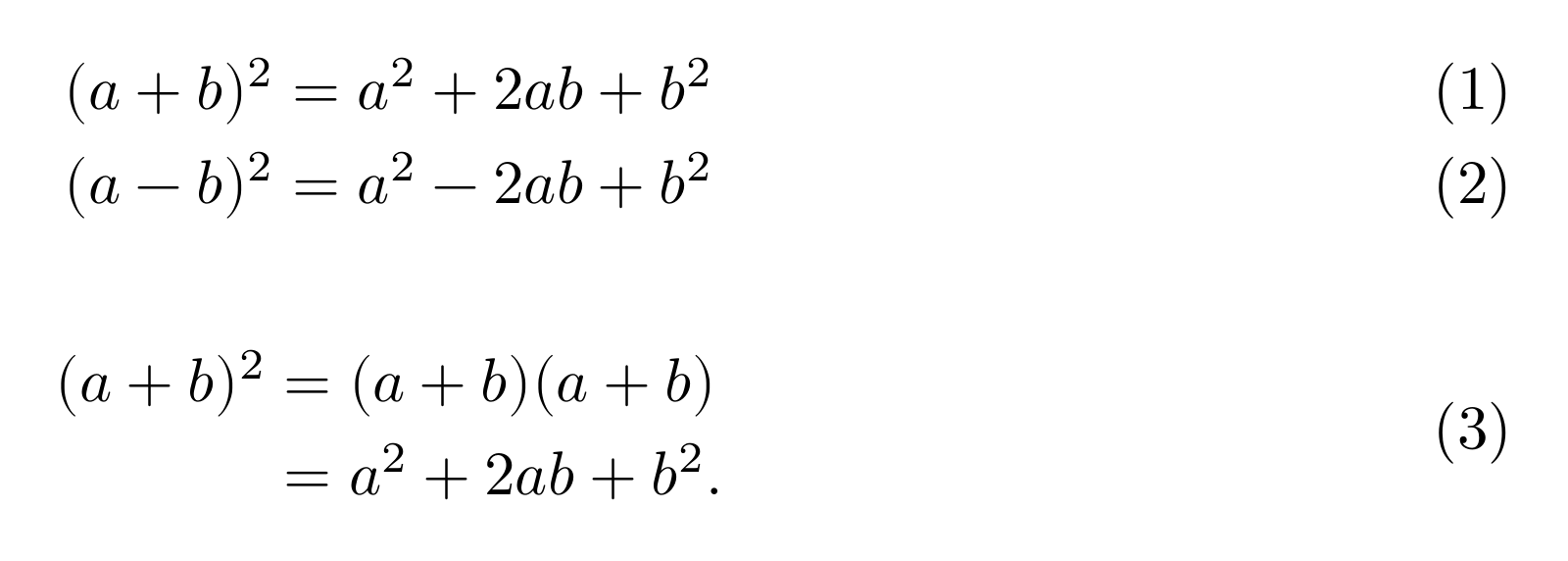
\begin{align}
  (a+b)^2 &= a^2+2ab+b^2 \label{eq:plus}\\
  (a-b)^2 &= a^2-2ab+b^2 \label{eq:minus}
\end{align}
For one number covering a whole derivation:
\begin{equation}
  \begin{aligned}
    (a+b)^2
      &= (a+b)(a+b)\\
      &= a^2+2ab+b^2.
  \end{aligned}
  \label{eq:expansion}
\end{equation}
A long unaligned expression can use multline:
\begin{multline}
  p(x)=a_0+a_1x+a_2x^2+a_3x^3\\
       +a_4x^4+a_5x^5+a_6x^6.
\end{multline}
multline left-aligns its first line, right-aligns its last, and centres intermediate lines. It does not use alignment markers.
IEEEeqnarray #
For finer control of mathematical columns, use IEEEeqnarray from IEEEtrantools:
% Preamble
\usepackage{IEEEtrantools}

% Body
\begin{IEEEeqnarray}{rCl}
  a & = & b+c \\
    & = & d+e.
\end{IEEEeqnarray}
Here the two & markers create separate left-hand side, relation, and right-hand side columns. \IEEEeqnarraymulticol spans columns, \IEEEeqnarraynumspace reserves room for a number, and \IEEEyessubnumber enables subnumbering. Ordinary align is sufficient for most calculations; do not substitute the older eqnarray environment, which has different spacing.
3.5 Units #
Units should be upright, consistently spaced, and formatted separately from mathematical variables. Load siunitx in the preamble:
\usepackage{siunitx}
Then use its structured commands:
A distance of \qty{12.5}{\metre}.
A speed of \qty{3.0e8}{\metre\per\second}.
An uncertainty of \qty{1.23(4)}{\metre}.
A number: \num{12345.6789}.
A unit alone: \unit{\kilogram\metre\per\second\squared}.
An angle: \ang{30;15;20}.
The uncertainty notation 1.23(4) denotes 1.23 with uncertainty 0.04. \numlist{1;2;3} and \qtylist{1;2;3}{\metre} format lists; \qtyrange{1}{5}{\second} formats a range. Set global options with \sisetup{...}, for example \sisetup{per-mode=symbol}.
Numeric table columns #
Use the S column type to align numbers by their decimal marker. Brace textual headings so they are not parsed as numbers:
% Preamble: also load booktabs
\usepackage{booktabs}

% Body
\begin{tabular}{@{}lS[table-format=3.2]@{}}
  \toprule
  Sample & {Mass (\unit{\gram})} \\
  \midrule
  A & 1.23 \\
  B & 12.30 \\
  C & 123.45 \\
  \bottomrule
\end{tabular}
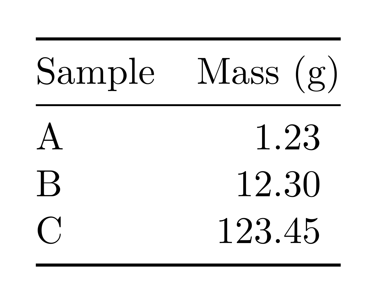
table-format=3.2 reserves space for three integer digits and two decimal digits. Include signs, exponents, and uncertainty fields in the specification when your data needs them.
3.6 Matrices and the Like #
Matrix cells are already in math mode. Separate columns with & and rows with \\:
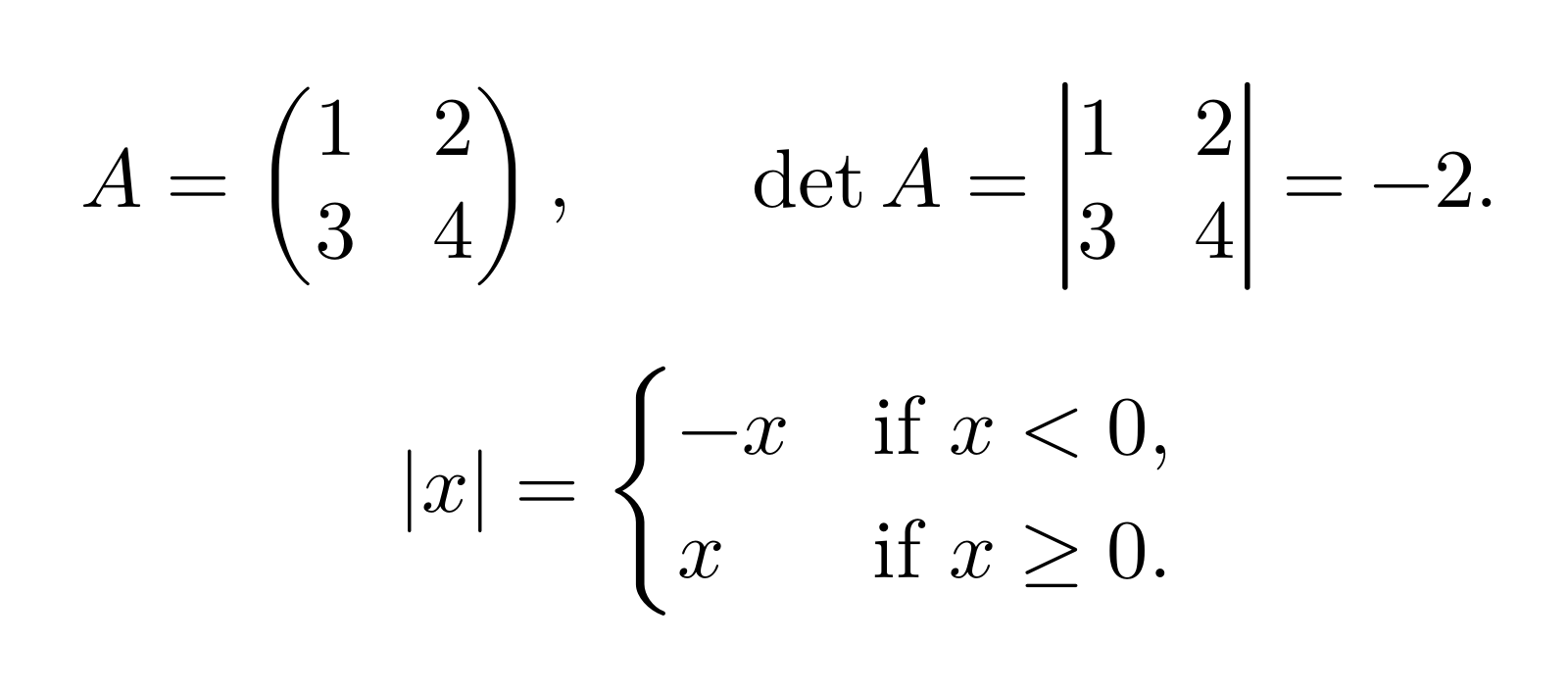
\[
  A=\begin{pmatrix}
    1 & 2\\
    3 & 4
  \end{pmatrix},
  \qquad
  \det A=\begin{vmatrix}
    1 & 2\\
    3 & 4
  \end{vmatrix}=-2.
\]
| Environment | Delimiters |
|---|---|
matrix |
None. |
pmatrix |
Parentheses. |
bmatrix |
Square brackets. |
Bmatrix |
Braces. |
vmatrix |
Single vertical bars. |
Vmatrix |
Double vertical bars. |
The smallmatrix environment fits small matrices into a line of text. array offers explicit column formatting inside math mode; matrix does not take a column specification. For a wider matrix, \setcounter{MaxMatrixCols}{12} raises the standard column limit.
Use cases for a piecewise definition:
\[
  |x|=\begin{cases}
    -x & \text{if } x<0,\\
     x & \text{if } x\geq 0.
  \end{cases}
\]
mathtools also provides dcases for display-style contents and starred matrix environments such as pmatrix* with optional column alignment.
3.7 Spacing in Math Mode #
LaTeX assigns spacing by mathematical role: ordinary symbol, operator, relation, opening delimiter, closing delimiter, or punctuation. Choose the correct command before adding manual spaces.
For a custom relation, define its role once:
% Preamble
\NewDocumentCommand{\related}{}{\mathrel{R}}

% Body
\(a \related b\)
Use \mathbin for a binary operator and \DeclareMathOperator for named functions. Do not put every relation in \text or align formulae with literal spaces.
| Command | Space |
|---|---|
\, |
Thin. |
\: |
Medium. |
\; |
Thick. |
\quad, \qquad |
One or two em-sized mathematical spaces. |
\! |
Negative thin space. |
\mspace{6mu} |
Explicit mathematical spacing. |
Phantoms reserve invisible space: \phantom preserves all dimensions, \hphantom only width, and \vphantom height and depth. They help match delimiters or align special notation. For left scripts, prefer \prescript{14}{6}{C} from mathtools over assembling them with empty groups and guessed spacing.
3.8 Theorems and Proofs #
Load amsthm and define theorem environments in the preamble:
\usepackage{amsthm}
\newtheorem{theorem}{Theorem}[section]
\newtheorem{lemma}[theorem]{Lemma}
\theoremstyle{definition}
\newtheorem{definition}[theorem]{Definition}
\theoremstyle{remark}
\newtheorem*{remark}{Remark}
The theorem counter resets with each section. Lemmas and definitions share it. The starred remark is unnumbered. The styles plain, definition, and remark distinguish statements, definitions, and commentary.
\begin{theorem}[Non-negativity]\label{thm:square}
For every real \(x\), \(x^2\geq 0\).
\end{theorem}

\begin{proof}
If \(x\geq 0\), the product \(x\cdot x\) is non-negative.
If \(x<0\), then \(x^2=(-x)^2\geq 0\).
\end{proof}
The proof environment adds an end-of-proof symbol. When a proof ends with a displayed equation, \qedhere can place the symbol on that final display.
3.9 Fiddling with Math Styles #
The four styles are \displaystyle, \textstyle, \scriptstyle, and \scriptscriptstyle. LaTeX selects them for displays, inline expressions, scripts, and nested scripts.
Override the style only when the automatic choice is unsuitable. A large inline fraction can disturb line spacing. \smash suppresses the recorded height and depth of its contents, but the ink is still there and can overlap other lines; it is a specialised tool, not a general cure.
3.10 Dots #
\dots adapts to nearby symbols. For precise control:
| Command | Context |
|---|---|
\dotsc |
Comma-separated lists. |
\dotsb |
Binary operators or relations. |
\dotsm |
Products. |
\dotsi |
Multiple integrals. |
\ldots, \cdots |
Explicit low or centred horizontal dots. |
\vdots, \ddots |
Vertical or diagonal matrix dots. |
\[
  A=\begin{bmatrix}
    a_{11} & \cdots & a_{1n}\\
    \vdots & \ddots & \vdots\\
    a_{n1} & \cdots & a_{nn}
  \end{bmatrix}.
\]
3.11 More About Fractions #
\frac follows the current style; \dfrac forces display size and \tfrac forces text size. \binom, \dbinom, and \tbinom do the same for binomial coefficients.
\[
  \sum_{k=0}^{n}\binom{n}{k}=2^n,
  \qquad
  \cfrac{1}{1+\cfrac{1}{1+\cfrac{1}{1+\dotsb}}}.
\]
\cfrac provides more suitable spacing for continued fractions. For small fractions in running text, 1/2 or \sfrac{1}{2} from xfrac may be preferable.
The general form is \genfrac{left}{right}{thickness}{style}{numerator}{denominator}. An empty style argument follows the surrounding style; 0–3 select the four mathematical styles. Define a meaningful wrapper rather than repeating this low-level construction:
% Preamble
\NewDocumentCommand{\stirlingfirst}{mm}{%
  \genfrac{[}{]}{0pt}{}{#1}{#2}%
}
Then \stirlingfirst{n}{k} typesets a bracketed two-level symbol without a fraction bar.