
6. Graphics in Your Document #
6.1 Overview #
Choose the representation to match the image:
| Material | Suitable format |
|---|---|
| Photographs | JPEG, with a suitable quality setting. |
| Screenshots, flat-colour raster drawings | PNG, which avoids lossy compression artefacts. |
| Diagrams, plots, and geometric drawings | Vector graphics, commonly PDF when included in LaTeX. |
Use graphicx for existing images. Use TikZ, built on PGF, when it is useful to describe a diagram in the document’s source: labels can use the same fonts and mathematics as the surrounding text, and repeated elements can share styles.
TikZ is not the only option. Specialised packages such as pgfplots for data plots can save substantial work compared with constructing every axis and tick manually.
All fragments in this chapter assume \usepackage{tikz} in the preamble. Additional libraries are named where they are needed.
6.2 Basic Usage #
A drawing lives in a tikzpicture environment. Drawing instructions end with semicolons:
\documentclass{article}
\usepackage{tikz}

\begin{document}
\begin{tikzpicture}
  \draw (0,0) -- (3,0) -- (1.5,2) -- cycle;
\end{tikzpicture}
\end{document}
(x,y) gives a Cartesian coordinate; units default to centimetres. (angle:radius) gives a polar coordinate, with the angle in degrees. -- draws a straight segment, and cycle closes a path with a proper join.
The general command is \path[options] ...;. \draw is shorthand for a path with the drawing action, \fill fills it, and \filldraw does both.
Nodes and coordinates #
Nodes contain ordinary LaTeX text or mathematics:
\begin{tikzpicture}
  \node[draw] (input) at (0,0) {Input};
  \node[draw] (output) at (4,0) {Output};
  \draw[->] (input) -- (output);
\end{tikzpicture}
The names input and output let later paths refer to the nodes. TikZ connects their boundaries rather than drawing through the text. Use anchors such as input.east or output.north to select a particular connection point.
\coordinate (A) at (1,2); names a point without creating a text box. A blank node still has padding, so it is not always interchangeable with a coordinate.
Add a label along a path:
\begin{tikzpicture}
  \draw[->] (0,0) -- node[above] {transform} (4,0);
\end{tikzpicture}
TikZ calculates a bounding box from the drawing. \useasboundingbox can specify an explicit box when you need consistent alignment between related pictures.
6.3 Curves and Shapes #
| Path operation | Meaning |
|---|---|
-- |
Straight line. |
-| |
Horizontal, then vertical. |
|- |
Vertical, then horizontal. |
to[out=30,in=150] |
Curve with specified departure and arrival angles. |
to[bend left] |
A bent connection. |
.. controls (A) and (B) .. |
A cubic Bézier curve. |
rectangle |
Rectangle between opposite corners. |
circle[radius=1cm] |
Circle around the current point. |
ellipse[x radius=2cm,y radius=1cm] |
Ellipse. |
grid[step=5mm] |
A grid between two corners. |
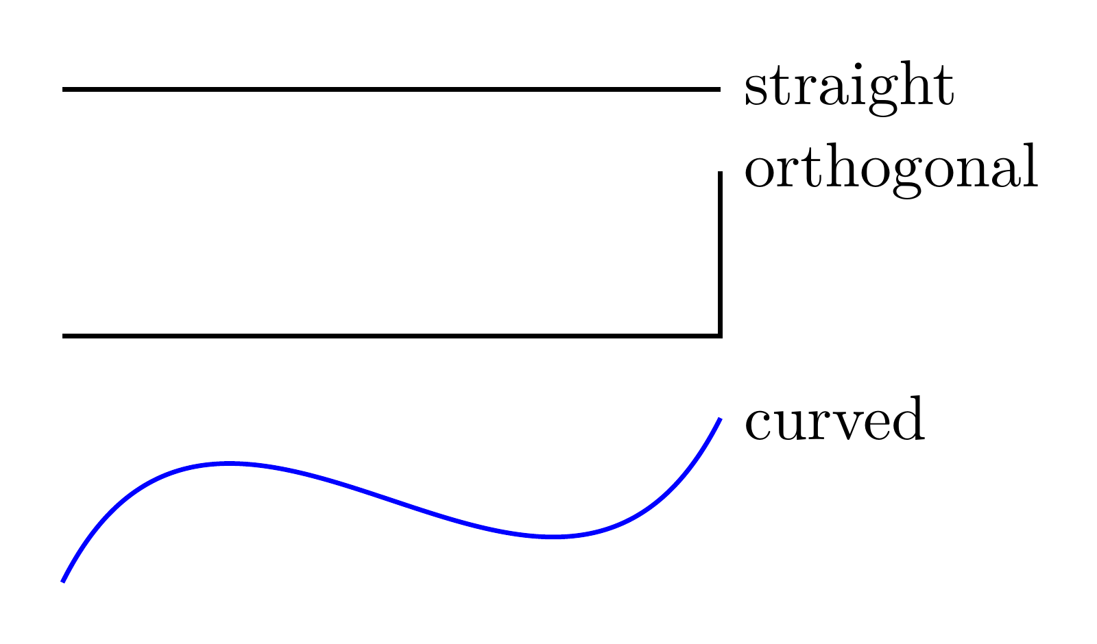
This example compares straight, orthogonal, and curved paths:
\begin{tikzpicture}[line width=0.8pt]
  \draw (0,2) -- (4,2);
  \node[right] at (4,2) {straight};

  \draw (0,0.5) -| (4,1.5);
  \node[right] at (4,1.5) {orthogonal};

  \draw[blue] (0,-1) .. controls (1,1) and (3,-2) .. (4,0);
  \node[right] at (4,0) {curved};
\end{tikzpicture}
An arc is described with a start angle, end angle, and radius:
\begin{tikzpicture}
  \draw (1,0) arc[start angle=0,end angle=90,radius=1cm];
\end{tikzpicture}
The coordinate before arc is the arc’s starting point, not the circle’s centre.
6.4 Customizing Paths and Nodes #
Options control appearance:
\begin{tikzpicture}
  \draw[blue,thick,dashed,->] (0,0) -- (3,1);
  \node[draw,fill=blue!10,rounded corners,align=center]
    at (1.5,-1) {Two lines\\of text};
\end{tikzpicture}
Use line width or names such as thin and thick for stroke weight; dotted or dashed for patterns; line cap and line join for ends and joins. Nodes can use draw, fill, circle, rounded corners, inner sep, and text width.
Set align when using \\ within a node. text width allows the text to wrap automatically.
Reusable styles #
Give repeated formatting a name:
% Preamble
\usetikzlibrary{arrows.meta,positioning}
\tikzset{
  processbox/.style={
    draw,
    rounded corners,
    fill=blue!8,
    minimum width=2.2cm,
    minimum height=9mm
  },
  flow/.style={-{Stealth},thick}
}

% Body
\begin{tikzpicture}[node distance=1cm]
  \node[processbox] (read) {Read};
  \node[processbox,right=of read] (write) {Write};
  \node[processbox,right=of write] (compile) {Compile};
  \draw[flow] (read) -- (write);
  \draw[flow] (write) -- (compile);
\end{tikzpicture}

Define styles in \tikzset for reuse across the document, or in the picture’s options for local use. every node/.style and every path/.style provide defaults within the current scope.
6.5 Coordinates #
Explicit units are allowed: (1in,12pt). The options x=1cm,y=5mm change the basis used by unitless Cartesian coordinates.
scale, xscale, yscale, rotate, xshift, and yshift transform coordinates. Scaling a picture’s coordinates does not normally scale node text; use transform shape when scaling node shapes and their contents is intended.
Relative coordinates reduce repetition:
\begin{tikzpicture}
  \draw (0,0) -- ++(0,1) -- ++(2,0) -- ++(0,-1) -- cycle;
\end{tikzpicture}
++(x,y) moves relative to the current point and updates it. +(x,y) gives a relative point without advancing the reference point.
Group related transformations in a scope:
\begin{tikzpicture}
  \begin{scope}[rotate=20]
    \draw (0,0) rectangle (2,1);
    \draw (0,0) -- (2,1);
  \end{scope}
  \begin{scope}[xshift=4cm]
    \draw (0,0) circle[radius=8mm];
  \end{scope}
\end{tikzpicture}
TikZ also accepts three-coordinate points and projects them using its x, y, and z basis vectors. This is a projection, not a complete three-dimensional scene renderer.
For a small drawing in a line of text, set baseline to control its vertical alignment, for example \tikz[baseline=-0.5ex]{\draw (0,0) circle[radius=0.7ex];}.
6.6 Reusing Pictures #
A pic is a reusable drawing inside another drawing:
\begin{tikzpicture}[
  marker/.pic={
    \draw[fill=blue!10] (0,0) circle[radius=3mm];
    \draw (-2mm,0) -- (2mm,0);
  }
]
  \pic at (0,0) {marker};
  \pic[red] at (1,0) {marker};
  \pic[scale=1.5] at (2,0) {marker};
\end{tikzpicture}
For a repeated pattern, use \foreach:
\begin{tikzpicture}
  \draw (0,0) circle[radius=1cm];
  \foreach \angle in {0,60,...,300} {
    \draw (0,0) -- (\angle:1);
    \fill (\angle:1) circle[radius=2pt];
  }
\end{tikzpicture}
Lists can also hold pairs, such as \foreach \x/\name in {0/A,1/B,2/C}. Keep the repeated geometry in one definition so a change applies consistently.
6.7 Libraries #
Load TikZ extensions with \usetikzlibrary rather than \usepackage:
\usetikzlibrary{arrows.meta,positioning,calc,intersections}
| Library | Adds |
|---|---|
arrows.meta |
Configurable arrow tips, including Stealth. |
positioning |
Relative node placement such as right=of A. |
calc |
Coordinate calculations. |
intersections |
Intersection points of named paths. |
external |
Caching drawings in separate files. |
With calc, ($(A)!0.5!(B)$) finds the midpoint of two coordinates and ($(A)+(B)$) adds their vectors.
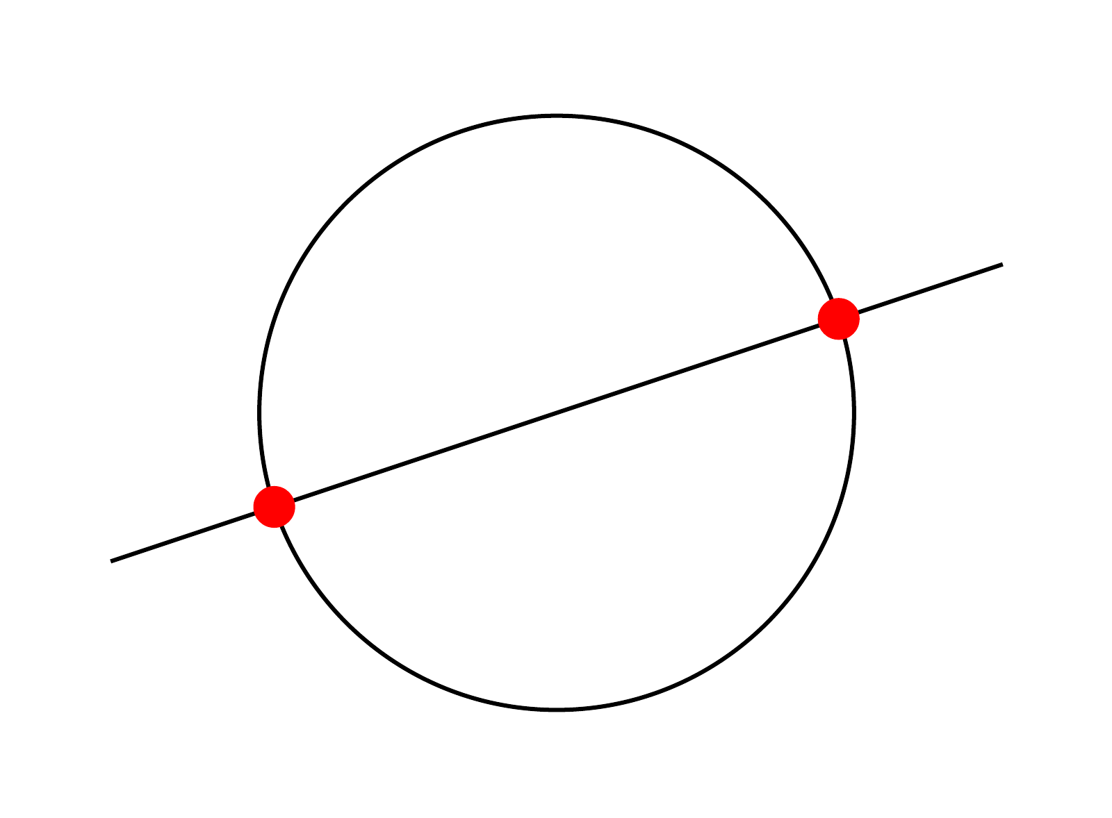
With intersections, let TikZ compute where a line meets a circle:
\begin{tikzpicture}
  \draw[name path=circle] (0,0) circle[radius=1cm];
  \draw[name path=line] (-1.5,-0.5) -- (1.5,0.5);
  \path[name intersections={of=circle and line}];
  \fill[red] (intersection-1) circle[radius=2pt];
  \fill[red] (intersection-2) circle[radius=2pt];
\end{tikzpicture}
Externalisation can reduce repeated compilation time:
% Preamble, after loading TikZ
\usetikzlibrary{external}
\tikzexternalize
It requires permission to launch the necessary external compilation commands and somewhere to write the generated files. On a restricted online compiler, check support before enabling it. An alternative is to compile a complex diagram separately and include the resulting PDF with graphicx.